SLAM and Kalman Filtering

This is initially a comparison between Kalman Filtering and SLAM for Platform/Vehicle Prediction and evolves into fleshing out a more usable and optimised SLAM system.

The SLAM code features additional custom edges (binary and unary) as well as vertices from the graph-based system (for vehicle and landmarks). Moreover, different systems can be iterated across and compared, via the flags described below and in the code. Furthermore, if the system hits a vertex which has an extremely high covariance (indicating a failed run and a bisected graph), the code will stop

and go into debug mode so that the user can see which vertex is faulty and garner more information. This should not happen during the tests provided.

The code for this project, including additional credits and details, can be found on my personal GitHub:

UPDATE: By request, to ensure academic integrity, this code has been removed.

The tasks carried out are as follows:

Part 1: Use pure Vehicle Odometry and compare the Kalman Filter and SLAM systems. Part 2: Include GPS for both KALMAN and G2o slam systems. Part 3: Implement the SLAM system to recognise landmarks and localise itself. Part 4.1: Add GPS to the new SLAM System. Part 4.2: Remove Vehicle Odometry from the system. Part 4.3: Graph Reduction - Graph Pruning is used. Random Graph Pruning (less effective) and sophisticated graph pruning (more effective) are toggled via flags.

The first task, using pure odometry leads to the following result:

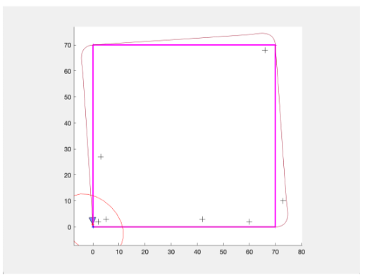
Where orange/red represents the Kalman Filter and Blue represents the SLAM system. The purple line shows the true path which the platform (blue triangle) takes. Notice how the prediction of the path is the same for both the Kalman Filter and the SLAM system and is exaggerated/inaccurate at corners. Furthermore, notice how the Kalman Filter prediction (red cross, bottom left) is slightly off from the true position whilst the SLAM (blue cross) system is correct. Finally, notice how the covariance ellipse is relatively large for both system, showing uncertainties.

When GPS is added into the same system, the following change was seen:

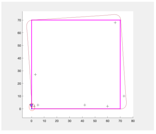
Notice how this does not necessarily increase the accuracy of the predicted path of either of the techniques, however, it does reduce the covariance (the ellipses in the bottom left) and hence the certainty of the systems. Additionally rates of GPS meaurements (1,2 and 5 seconds) were tested too.

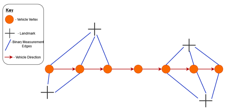
After this, the whole SLAM system was implemented (landmark detection and re-optimisation) on a new, more complex map. Below, an indication as to how the SLAM graph was built is given:

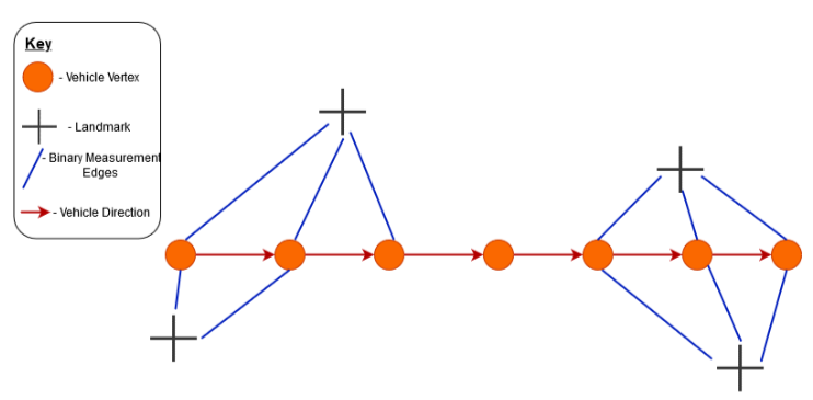
All vertices and edges were created as part of the graph-building SLAM algorithm which I wrote (and then optimised to reduce errors using G2o's core optimisation). Another system using unary edges for landmarks and optimising from MATLAB first-principles was also implemented. On the more complex graph, this leads to the following results

On the left, the system without GPS is shown, and on the right the sytem with GPS is shown. Notice that the main difference between the two is the drastic change in covariance - the additional GPS measurements remove uncertainty from the system. The black crosses show the true landmarks and the blue dots/ellipses show the SLAM's prediction of these landmarks. Notice how a non-trivial number of the landmarks which are set far from the vehicle's path are not detected or badly predicted, although closer landmarks are predicted well.

In the case above, all odometry edges/measurements are still included and factor into the prediction. However, with the individual landmark detection now working (and noting that each landmark has a unique ID, which in real life would distinguish landmarks from one another), the odometry edges are likely unnecessary and removing these edges can result in a reduced graph, easing the computational itnesity and speed of the system. Therefore, all vehicle odometry edges are deleted (except the first one, since this is used to place the vehicle's starting position in the World) and GPS measurements are taken every second, which leads to the following results:

As can be seen above, this is more accurate than the previous systems - this is aminly due to an increase in the range of the vehicle's detection of landmarks, which allows for distant landmarks to be seen multiple times. Removing odometry measurements does not necessarily increase the accuracy of the system (as the above can be found by using the same range and GPS settings with odometry edges), in fact it may cause some small sporadic errors, but it does reduce the graph size, as the below statistics show:

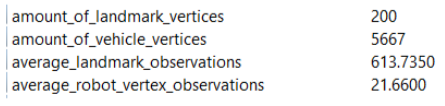
Hence, removing al but one odometry edge removes 5666 measurements from the system, each of which must be individually optimised, vastly reducing the computational intensity of this system, allowing it to further approach real-time.

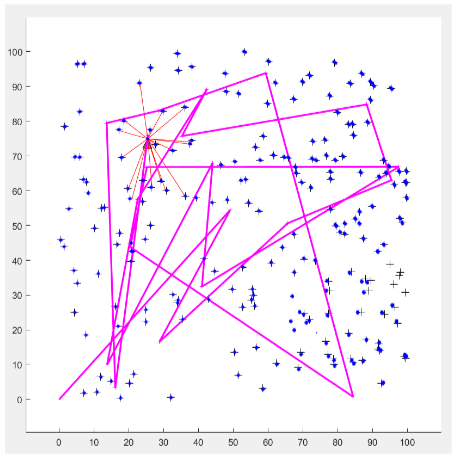
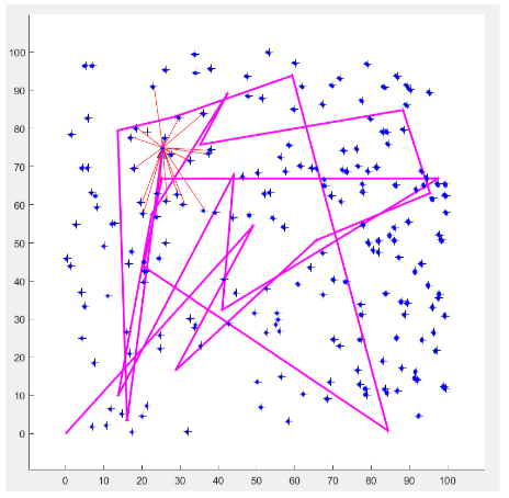
Finally, graph pruning was implemented. Up until now, all measurements/sightings of the landmarks from the vehicle have been included in the optimisation, however, not all of these are necessary in finding the landmarks and reducing the number of landmark measurmeents (pruning the graph) can reduce the computational complexity and can have impacts on the accuracy too. Initially, landmark measurement edges were randomly deleted, however, with no odometry edges this leads to bisection - an example is given below:

Notice how the graph has split into two separate graphs (left and right), and with no odometry edges, there is no way to relate the second graph to the original odometry edg, locating the SLAM system in the world, and hence the edges cannot be optimised - the system fails. Therefore, it was imperative that I created a system which made sure that bisection was not possible (ie making sure that each consecutive vehicle vertex had landmark detections in common with the one before and the one after itself).

This means that there is a "core" graph which is necessary - where only landmark detection edges which preserve connectivity (ie prevent bisections) are present and all others are deleted. Any additional landmark detection edges added onto this core graph is then only to increase optimisation accuracy. This variable of "additional" edges wasadded into the system I created, which led to the following results:

The graph on the left shows the results when at least 5 additional landmark measurement edges per vehicle vertex are included, whereas the right hand side graph shows the results when 10 additional landmark edges are included. Each of these results omits GPS (hence the large covariance ellipses), for ease of computation. As can be seen above, the accuracy of the 10 edge inclsuion is far superior to the 5 edge inclusion, since it correctly predicts all landmarks, which the other does not. This analysis is abotu balancing accuracy with graph size and the right hand side graph (10 edges included) reduces the graph whilst not compromising accuracy. The graph reduction results are shown below:

Again, the left shows the 5-edge inclusion results and the right shows the 10-edge inclusion results. Whilst the 5-edge inclusion does reduce the graph by more, based on the statistics above, he graph reduction is not worth it when compared to the potential accuracy concessions, and hence all things considered, the 10-edge inclusion case was chosen as optimal.

Finally, this means that with this sophisticated graph pruning and removal of odmometry edges, the inclusion of the GPS system leads to the following final system:

This shows a highly accurate, low covariance system, with a reduced graph to optimise computational efficiency - this is highly desirable for modern SLAM systems.