Multi-Agent DQN Implementation

Recently, I have implemented a multi-agent DQN (Deep Q Network) system - this is classified as a Multi-Agent Reinforcement Learning system (MARL). In order to test the capabilities of multi-agent DQNs, they were used in order to play the Switch_v2 game from ma-gym.

DQNs are a value-based reinforcement learning method where the Q table, in conventional Q-learning, is replaced by a neural network, which can find patterns and generalise over a large amount of inputs - an amount which would conventionally lead to a Q table which was too large and sparse to be of much practical use - this is the power of DQNs.

Two individual DQNs were implemented and neither had any connection to the other - ie each agent did not know any information about the other agent. In this wholly secular approach to multi-agent reinforcement learning, each agent simply sees the other agent as a "part of the environment" and another obstacle to navigate to reach its goal - in the switch_v2 game, this goal is for each agent to reach a specific point on the map. Each agent spawns on the other side of the map and the map features a corridoor to reach the other side of the map, however, the corridoor is only one unit wide and hence only one agent at a time can fit through it. Therefore, for this system to optimise its reward, there must be a form of cooperation between the systems, even though they have no method of communication - the durability of DQNs allows for this optimisation.

My implementation can be seen below (using Jupyter's nbviewer) and on my GitHub here:

https://github.com/RayDanks/DQN_Switch_v2/blob/master/DQN_Switch_v2_Implementation.ipynb

Scroll bars are given at the bottom of each cell below, although the above GitHub repository allows for better viewing and formatting of the implementation.

The results from my implementation are shown in graph form below:

Firstly, the learning curve:

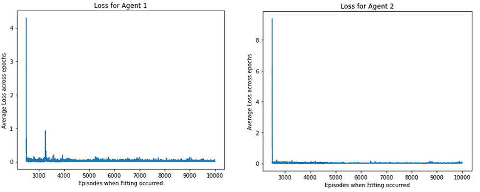
Secondly, both the agents' loss graphs (note that this just shows how well each network conforms to the given policy, not how good that policy is):

Below I have written some analysis on the above results and on the general behaviopur of my specific multi-agent DQN implementation:

Method: I implemented Deep Q Networks (DQNs) to play the switch_v2 game. The only input to these networks are the agents’ independent states, along with the timestep. I used an individual ANN for each network, which was routinely fitted by random sampling from an experience replay. This was done at regular intervals, instead of after each action, in an attempt to keep the data i.i.d. Before fitting begins, the agents are allowed to explore the environment randomly, in order to adequately fill the replay memory. This stops the agents taking the first plausible strategy and getting stop in a local minimum. Effectiveness/Results: The results can be seen in the Learning Curve, the two Loss Graphs and the Testing Phase.

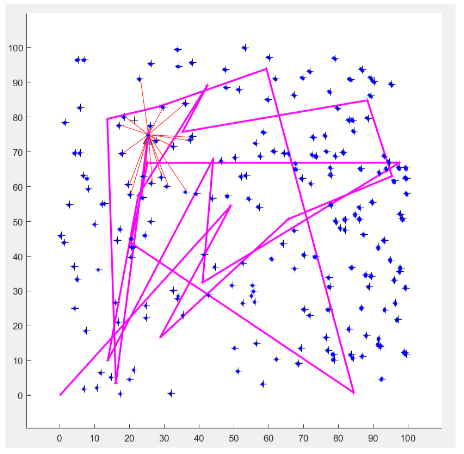
Testing: The system was tested by just drawing actions from the networks/trained policies (no exploration) and visualising the system. The system does not always work, due to randomness(and other defects described here), although it often works and the Learning Curve shows that it does learn adequately.

Analysis: The system works well – it achieves a solution which satisfies the reward criteria in an effective manner, taking advantage of the timestep information provided to the networks in a manner such that one agent waits for the other to complete the course before they start their action. The optimal minimum number of steps to complete is 13, and this system regularly gets close to this optimum. This is verified by the visual video, along with the graphs provided.

The Learning Curve is intriguing, my method of training plateaus the system at a relatively high epsilon, so that it can learn not to get stuck in local minima. This, along with the relative disparate of the system (due to the lack of a target network perhaps) means that the reward seems to oscillate between episodes, although the maximum reward increases, showing that learning is occurring. Target Networks, full grid-searching hyperparameter optimisation, target frequency optimisation and the like would remove this uncertainty/oscillation within the system. Even when the system fails, visualising the movement shows that the two agents are just out of time with one another and get stuck in the corridor, meaning that they have already learned their own strategies (they are not moving randomly) but have badly estimated the timestep aspect. This shows that each agent is learning well.

The loss function graphs offer good insight into the inner workings of the system. The small oscillation on the loss graph is as expected, since the policy is constantly changing. If the loss graphs were to show spikes, this could be indicative of exploding gradients, which can imply that the agent has hit a local optimum/results that are unexpected and hence the policy has changed dramatically (ie when the agent gets stuck in the corridor). Gradient Clipping can often remedy this. The lack of spikes in my loss graphs shows that they each conform to a global minimum and optimal policy well.

Finally, here are some extra resources which are informative about DQNs and MARL in general and also helped me to understand many of the conceots pertaining to these techniques too:

Mnih, V., Kavukcuoglu, K., Silver, D. et al. Human-level control through deep reinforcement learning. Nature 518, 529–533 (2015). https://doi.org/10.1038/nature14236

https://keras.io/callbacks/ (For Loss History Class)

https://medium.com/@jonathan_hui/rl-dqn-deep-q-network-e207751f7ae4

https://pythonprogramming.net/training-deep-q-learning-dqn-reinforcement-learning-python-tutorial/?completed=/deep-q-learning-dqn-reinforcement-learning-python-tutorial/

https://towardsdatascience.com/dqn-part-1-vanilla-deep-q-networks-6eb4a00febfb

https://www.analyticsvidhya.com/blog/2019/04/introduction-deep-q-learning-python/